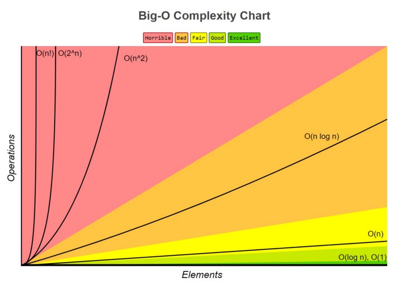
Time complexity

Time complexity (also runtime complexity) is an evaluation of the runtime (usually number of operations) of a given algorithm. We commonly express complexity in terms of big-O notation (more broadly asymptotic notation). Algorithm time requirements are described in terms of the size ($n$) of the problem instance.

Big O refers to the upper bound on an algorithm’s runtime. Big-omega refers to the lower bound. If big-omega and big-O are the same, then we use big-theta notation (which is like a tight upper/lower bound limit). We say that a function $f(n)$ has time complexity $O(g(n))$ if there’s a

Many problems, like the travelling salesman problem, have a time complexity of $2^n$, i.e., we can only solve for small values of $n$. Problems like this are NP-hard, and are important topics of research in theoretical computer science.

Finding big-O

We drop constants and coefficients¹ — i.e., $O(2n)$ is expressed as $O(n)$. $n$ just describes the rate of increase. The lesser terms are dropped as well. To summarise, take $f(n)=6n^4-2n^3+5$ as an example. We can just express as $O(n^4)$.

If the algorithm looks like: “do this, then when done, do that”, we can add the runtimes: $O(A+B)$. If it looks like “do this for each time you do that”, then we multiply the runtimes: $O(A\cdot B)$. If our algorithm reduces the operating size by dividing (i.e., halves the search array), then we have $O(\log n)$ time.²

For recursive algorithms, it’s a good idea to use a recurrence expansion. Oftentimes in recursive algorithms when we run into a “tree” (not in the binary tree sense, in the “how does the computation expand” sense) that expands as $n$ increases, we deal with $O(a^n)$, where $a$ is the number of child branches that get split each time. Generally: $O(\text{branches}{)}^{\text{depth}}$.

For binary search trees, we divide the search set in half each time. If we do two operations (for each sub-tree) per cycle (like printing), then we effectively run into $O(2^{\log n})$, which reduces into $O(n)$. The algebra is a little funky here but this is true and provable.

This is also true for the worst-case complexity for searching regular trees!

In software engineering

Why does this matter? As software engineers, we can’t always brute force a solution — sometimes we have finite computational resources. This helps us understand the idea of code efficiency (again very important in embedded and server code). There usually isn’t a single algorithm that is fastest in all cases. So we have a best case, expected case, and worst case scenario.

Usually the expected case and the worst case are the same.

The runtime of a program depends on computer speed and power, the compiler, the programming language, the nature of the data, and the size of the input. We’re interested in building algorithms that perform well with respect to input sizes irrespective of hardware limitations. The right algorithm can make slower computers perform better than faster computers for larger $n$.

Performance is less important than:

• Correctness
• Maintainability
• Modularity
• Functionality
• Extensibility
• Security
• User-friendliness
• Scalability
• Robustness

It’s important not to start optimising programs too early. Often we can predict poorly which areas will act as performance bottlenecks, so code is sometimes optimised too early or unnecessarily by programmers, which leads to complex and buggy programs that don’t work the way they’re supposed to.

It’s better to write a simple, correct program, then analyse its performance and optimise later.

Resources

• Cracking the Coding Interview, by Gayle McDowell, is an excellent introductory resource to finding big-O without the rigour of CLRS
• Introduction to Algorithms by CLRS is, as always, a quintessential rigorous exploration of complexity analysis

Footnotes

1. Because the constants are largely swamped out by the actual function with realistic input sizes. ↩

2. What’s the base? It usually doesn’t matter, because $\log$ is differentiated only by a constant factor, i.e., ${\log }_{4}x=\log x/\log 4$ ↩