Bellman-Ford algorithm

The Bellman-Ford algorithm is a graph traversal algorithm that solves the shortest path problem. It can process most graphs, provided it doesn’t contain a cycle with negative length.

Basics

The algorithm works by keeping track of the distances from the starting node to all nodes of the graph. Initially, the distance to the starting node is 0, and to other nodes is infinite. By finding edges that shorten the path, this reduces the distances until it’s not possible to continue reducing.

It relies on $v-1$ passes, i.e., we relax each edge $v-1$ times. From an infinite initial state, it only takes weights that reduce the distance to a given node. The overall time complexity is $O(VE)$, because it takes $v-1$ passes and iterates through all $E$ edges during a round.

In this sense, the Bellman-Ford algorithm is a dynamic programming algorithm.

Implementation

for (int i = 1; i <= n; i++)
	distance[i] = INT_MAX;
distance[x] = 0;
for (int i = 1; i <= n - 1; i++) {
	for (auto e: edges) {
		int a, b, w;
		tie(a, b, w) = e; // tuple of references
		distance[b] = min(distance[b], distance[a] + w);
	}
}
for (auto e: edges) {
	if (e.first > e.second + e.weight) // negative weight cycle
		return false;
}
return true;

Applications

Bellman-Ford can also check for a cycle with a negative length within the graph. Because of the way BF is structured, we can infinitely shorten any path that contains the cycle by repeating the cycle again and again. If we run it for $n$ rounds and the last round reduces distance, the graph contains a negative cycle.

As a distance vector algorithm

In computer networking, Bellman-Ford functions as a distance vector algorithm in the control plane. It is a distributed algorithm, mainly because each node functions by computing the distances to the next nodes (computation diffuses information through the network), and also because it’s largely asynchronous.

If we define $x$ as the node, and $y$ as another node in the network, then the function below describes the minimum distance from $x$ to $y$.

$$D_x(y)=\underset{v}{\min }\{c_{x,v}+D_v(y)\}$$

From time-to-time, each node will send its own distance vector estimate to its neighbours.

• $x$ receives a new DV estimate from any neighbour.
• It updates its own DV using the Bellman-Ford equation.
  • Eventually, the estimate $D_X(y)$ will converge to the actual least cost $d_X(y)$.
• If the DV to any destination has changed, the node will send its new DV to neighbours.
  • If no change is necessary, then no actions need to be taken!
  • Thus, the algorithm systemwide will terminate eventually.

Analysis-wise:

• In terms of message complexity, since there’s an exchange between neighbours, the convergence time varies. The speed of convergence varies, as there may be routing loops, or the “count-to-infinity” problem.
• Suppose a Byzantine failure scenario: what if a router malfunctions or is compromised?
  • A DV router can advertise an incorrect path cost. This is called black-holing.
  • The error will propagate through the network.
  • i.e., it is not Byzantine fault tolerant.

Problems

As with many distributed algorithms, it is slow for information to propagate fully and converge (consider how low the throughput of Paxos is). A routing loop happens when a link cost increases. This essentially results in a situation where a packet is bumped between the same group of routers, since the routers haven’t updated their link costs (stuck in a local minima, so to speak). Each node’s estimated costs will keep incrementing as the nodes exchange information, until it breaks out of the loop. This is the count-to-infinity problem: basically good news (reduction in link costs) travels quick, but bad news (increase) travels slow.

There are two mechanisms where this can happen:

• A routing loop happens when a link cost increases, and results in a packet being bumped between router to router making no progress in the network. Each node thinks there’s a better path through the other node. Eventually, they increment their costs (like gradient descent) until they reach the true cost and the packet escapes the loop. This is finite.
• Another is a network partition (also called split horizon) between nodes. By this point, the distance between partitioned nodes is $\infty$, but the nodes in each segment of the network don’t know this. Instead, they keep incrementing to $\infty$, which adds extra load onto the network.

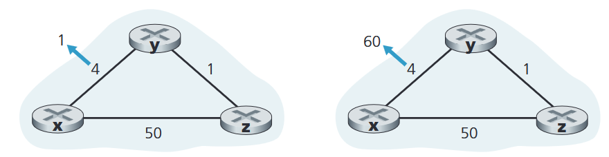
Concretely, consider this example, where the link cost between nodes $x,y$ increases from 4 to 60.

• In iteration 1 after the link cost change:
  • $y$ detects the link cost to $x$ is now 60.
  • $y$ computes: $D_y(x)=\min \{60,1+D_z(x)\}=\min \{60,1+5\}$.
  • $y$ routes through $z$, assuming it can reach $x$ with cost 5.
  • $y$ advertises its new distance vector to node $z$.
• In the next iteration:
  • $z$ receives $y$‘s distance vector, and that $D_y(x)=6$.
  • $z$ computes $D_z(x)=\min \{50,1+D_y(x)\}=\min \{50,1+6\}$.
  • i.e., $z$ now thinks it should go through $y$ to reach $x$.
  • $z$ advertises its new distance vector to $y$.
• And this continues for 44 iterations until the path cost reaches the true cost.

See also

• Dijkstra’s algorithm, a greedy algorithm for the shortest-path problem
• A-star algorithm, a heuristic algorithm for the shortest-path problem
• Floyd-Warshall algorithm