Continuous-time Fourier transform

The continuous-time Fourier transform (CTFT) is an integral transform that allows us to perform Fourier analysis (which was previously restricted to periodic signals) on aperiodic signals.

The CTFT of a CT signal $x$ is the complex-valued signal $X:\mathbb{R}\to \mathbb{C}$ defined by:

$$X(j\omega )={\int }_{-\infty }^{\infty }x(t)e^{-j\omega t}dt$$

where $X$ is the Fourier transform or spectrum of $x$. The inverse CTFT of a CT spectrum $X$ is the CT signal $x:\mathbb{R}\to \mathbb{C}$ defined by:

$$x(t)=\frac{1}{2\pi }{\int }_{-\infty }^{\infty }X(j\omega )e^{j\omega t}d\omega$$

If $x$ is a periodic signal (with fundamental period $T_0$), the CTFT spectrum is given by:

$$X(j\omega )=2\pi \sum _{k=-\infty }^{\infty }{\alpha }_k\delta (\omega -k{\omega }_0)$$

Computations

A windowing function will produce a sinc function in the opposite domain:

$$x(t)=u(t+3)u(3-t)\to X(j\omega )=\frac{\sin (3\omega )}{\omega /2}$$

There isn’t an immediate formulaic way (I think) to find this (depends on the circumstance) but windowing functions are fairly easy to find the CTFT of.

Properties

If $x$ is very concentrated in the time domain, it will be very spread out in the frequency domain. Additionally, a multiplication of functions in the time domain is a convolution in the frequency domain.

In general, any real-valued signal $x$ will have a spectrum $X(j\omega )$ with conjugate symmetry, i.e., $X(j\omega {)}^{\ast }=X(-j\omega )\forall \omega \in \mathbb{R}$. Then we have two results:

• The magnitude $|X(j\omega )|$ is an even function of $\omega \in \mathbb{R}$.
• The phase $\angle X(j\omega )$ is an odd function of $\omega \in \mathbb{R}$.

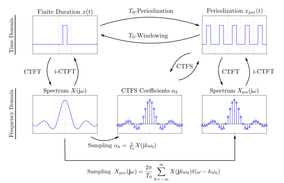
The relationship with the CTFS is as follows:¹

Existence

If $x$ has finite action, i.e., $x\in {\mathsf{L}}_1$, then the CTFT $X(j\omega )$ is well-defined and satisfies ${\lim }_{\omega \to \pm \infty }|X(j\omega )|=0$. The proof for the well-defined statement is given by:

$$|X(j\omega )|=|{\int }_{-\infty }^{\infty }x(t)e^{-j\omega t}dt|\le {\int }_{-\infty }^{\infty }|x(t)|\cdot |e^{-j\omega t}|dt={\int }_{-\infty }^{\infty }|x(t)|dt$$

For the second statement, the proof is given by the Riemann-Lebesgue lemma.

Additionally, if $x$ has finite energy, i.e., $x\in {\mathsf{L}}_2$:

• Then $X$ exists and has finite energy, i.e., $X\in {\mathsf{L}}_2$.
• The signal and its spectrum satisfy Parseval’s theorem.

In either case, the signal may not have finite action nor finite energy, i.e., $x\notin \{{\mathsf{L}}_1,{\mathsf{L}}_2\}$ but still have a CTFT. For example, the complex exponential signal $x(t)=\exp (j{\omega }_{0}t)$ has CTFT $X(j\omega )=2\pi \delta (\omega -{\omega }_0)$.

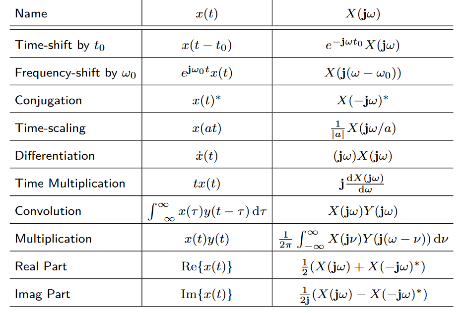
Table of properties

Derivation

If we have an aperiodic CT signal $x(t)$, we take a few steps. We first window a signal between a period $[-T,T)$ to obtain a finite-duration signal, which we then periodise.

$$x_{\text{fin}}(t)=x(t)[u(t+T)-u(t-T)]$$ $$x_{\text{per}}(t)=\sum _{m=-\infty }^{\infty }{x}_{\text{fin}}(t-m(2T))$$

When we represent it with the CTFS:

$$x_{\text{per}}(t)=\sum _{k=-\infty }^{\infty }{\alpha }_k{e}^{jk{\omega }_{0}t}$$ $${\alpha }_k=\frac{1}{2T}{\int }_{-T}^{T}x(t)e^{-jk{\omega }_{0}t}dt$$

If we define a complex-valued function:

$$X_T(j\omega )={\int }_{-T}^{T}x(t)e^{-jk{\omega }_{0}t}dt$$

Then the CTFS coefficients are samples of $X_T$:

$${\alpha }_k=\frac{1}{2T}{X}_T(jk{\omega }_0),k\in \{-\infty ,\cdots ,\infty \}$$ $$x_{\text{per}}(t)=\frac{1}{2\pi }\sum _{k=-\infty }^{\infty }{X}_T(jk{\omega }_0)e^{jk{\omega }_{0}t}{\omega }_0$$

Since $T=\pi /{\omega }_0$. Since this sum functions as a Riemann sum with representative width ${\omega }_0$, we can generalise as $T\to \infty$, such that:

$$x(t)=\frac{1}{2\pi }{\int }_{-\infty }^{\infty }X(j\omega )e^{j\omega t}d\omega$$ $$X(j\omega )={\int }_{-\infty }^{\infty }x(t)e^{-j\omega t}dt$$

Footnotes

1. From Prof Simpson-Porco’s lecture notes. ↩