Frequency response

In system theory, the frequency response describes how a given system processes signal components at different frequencies: how their amplitudes are scaled, phases are modified, and so on. The frequency response is described by the CTFT of a system’s impulse response:

$$H(j\omega )={\int }_{-\infty }^{\infty }h(t)e^{-j\omega t}dt=H(j\omega )=|H(j\omega )|e^{j\angle H(j\omega )}$$

where $H(j\omega )\in \mathbb{C}$. There are three main properties that tell us an LTI system will amplitude-scale and phase-shift any complex exponential input:

• Eigenfunction property — for $x(t)=e^{j{\omega }_{0}t}$, $y(t)\propto e^{j{\omega }_{0}t}$.
• Amplitude scaling — the output amplitude is scaled by $|H(j{\omega }_0)|$.
• Phase shifting — the output phase is shifted by $\angle H(j{\omega }_0)$.

We can obtain the frequency response from the system’s transfer function $H(s)$ only if the Laplace transform exists for a given value of $s$, i.e., $\text{Im}(s)\ne 0$. By substituting $s=j\omega$, any computations we do to find a given transfer function can be used to find the frequency response.

For a system with a transfer function $T(s)$ driven by an input function $x(t)$, we define its steady-state response $y_{ss}(t)$ as the function $y(t)$ converges to as $t\to \infty$.

$$y_{ss}(t)=x(t+\angle T(j\omega ))\cdot |T(j\omega )|$$ $${\text{Y}}_{ss}=|x(t)|\cdot |T(j\omega )|(\angle x(t)+\angle T(j\omega ))$$

The transient response of the system converges, i.e.,:

$$\underset{t\to \infty }{\lim }[y(t)-y_{ss}(t)]=0$$

For a sinusoidal input signal, we have a few key properties for the steady-state interpretation of the response:

• The output response to a sinusoidal input is also sinusoidal.
• The response has the same frequency as the input.
• The response amplitude is the input amplitude times the $|H(j{\omega }_0)|$.
• The response phase is the input phase plus a shift of $\angle H(j{\omega }_0)$.

Terminology

There are three big terms, annotated on this gain plot (a frequency diagram):¹

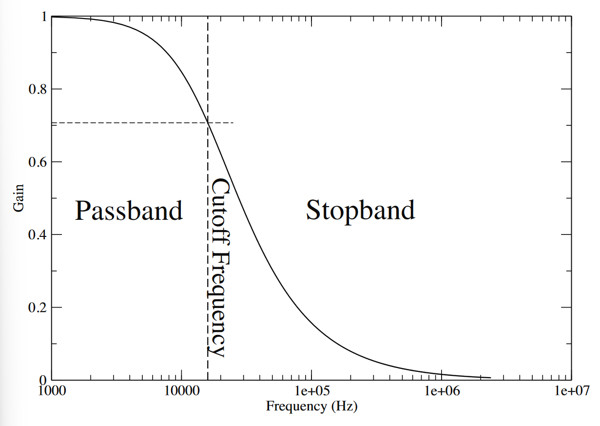
• The cut-off frequency is the frequency at which the gain is reduced from its maximum value by a factor of $\frac{1}{\sqrt{2}}=0.707\dots$
• The stopband describes the region of the plot where the gain is significantly reduced.
• The passband describes the region where the gain is fairly high.

Both the stopband and the passband can exist in high or low frequency regions. We encounter four types of frequency response, the first two being first-order and latter two being second-order:

• A low-pass response has a low frequency passband and a high frequency stopband.
• A high-pass response has a high frequency passband and a low frequency stopband.
• A bandpass response has one passband in the centre, surrounded by two stopbands.
• A bandstop response has one stopband in the centre, surrounded by two passbands.

A meaningful way to plot the frequency response is through Bode plots, since we can sufficiently zoom in. More on that over there.

Related links

• Bandwidth

Footnotes

1. From Prof Najm’s notes, lecture 28. ↩