Operational amplifier

Operational amplifiers (op amps) are differential amplifiers with a very large open-loop gain $A$ (usually around $10^5$ to $10^8$). The “operational” in their name comes from the circuits they’re used in, where they are used to do operations on signals.

The theory gets a little dense, but the ideal case is easier to work with. Really cool IMO. Prof Najm’s lectures on what you can do with these were so eye-opening.

Ideal model

We use a few simplifying assumptions for ideal op amps:

1. The linear gain $A$ is approximately infinite.
2. The input resistance $R_{\text{in}}$ is infinite, so $i_{\text{in}}=0$. So any branches connected to it will not have any current pass to the op amp.
3. The output resistance $R_{\text{out}}=0$.

The ideal op amp model is given by the below symbol. The - terminal ($v_n$) is the inverting input, and the + terminal ($v_p$) is the non-inverting input. 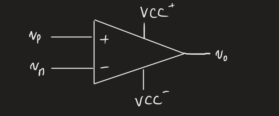Because $R_{\text{in}}$ is approximately infinite, we have it such that $v_p=v_n$. When in a feedback configuration, this creates a virtual short circuit between the +/- terminals. This is an important implication, because if one terminal is connected to ground, we have the other terminal at ground (even if it’s connected to a circuit), a virtual ground.

Analysis with the ideal model is pretty simple. Write out the equations for the simplifying assumptions and spam KCL.

Real model

In the real model, our simplifying assumptions get a little fuzzier:

• The gain $A$ is really high ($A\approx 100000000$), so the transfer characteristic is almost vertical in linear mode, but not quite.
  • There’s no need for a gain this high, because amplifying a tiny signal isn’t really useful and there’d be too much noise. We instead use op amps in combination with other elements to deliver more moderate gains — and also more stable and flexible circuits.
• The input resistance is large, around $10^6$ to $10^{12}$ Ω.
• The output resistance is small, around 10 to 100 Ω.

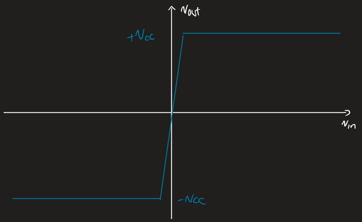
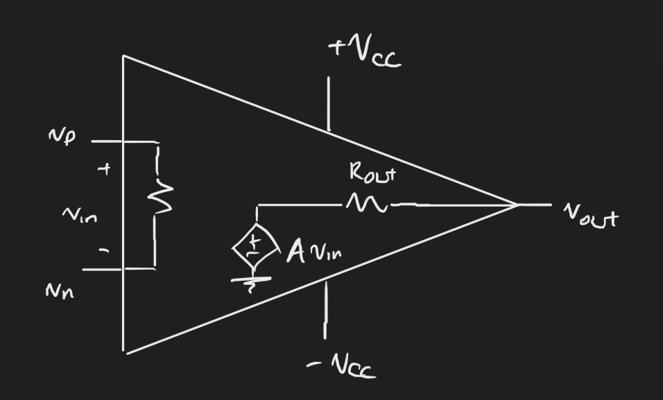
The real transfer characteristic is given by: We model op amps in linear mode with:

Non-linearities

One problem with op amps at DC is the input offset voltage ($V_{OS}$), i.e., for an input voltage at a certain terminal, the other terminal will be offset by a small amount. This includes if one terminal is grounded — we will see a slight DC voltage at the output.

For the op amp to operate, both input terminals must be supplied with DC currents called the input bias currents. Why does this make sense? (since the ideal op amp had $i_{\text{in}}=0$) Since the input resistance is finite, there’s a small (a few nanoamperes) current passing through. The input bias current is given by the average value of each terminal, and the input offset current is given by the difference:

$$I_B=\frac{I_{B1}+I_{B2}}{2}$$ $$I_{OS}=|I_{B1}-I_{B2}|$$

In large signal operation, there are several limitations on op amp functionality. The op amp will reach saturation, where it reaches past the absolute maximum of its rated performance at the rated output voltage (in many cases less than the supply rails). When the op amp saturates, the output signal peaks will be clipped off.

Output current is also limited to a specific maximum. If the circuit requires more than a certain amount of rated current, the op amp will saturate.

The slew rate (SR) is the maximum rate of change possible at the op amp’s output. It’s given by:

$$\text{SR}=\frac{d{v}_o}{dt}{|}_{\text{max}}$$

What this means is that for a given intended rate of change, the op amp will only function at its slew rate if the input rate is larger than what it can support. This can result in distorted output waveforms.

Frequency response

The ideal op amp model doesn’t take frequency into consideration. In reality, the differential open-loop gain $A$ decreases with frequency. When op amps are connected in a feedback configuration, we get more stable circuits with an increased bandwidth. This results in the op amp being much more useful in signal filter design.

Below is a graph of the typical frequency response of op amps on the market (like the μA741).

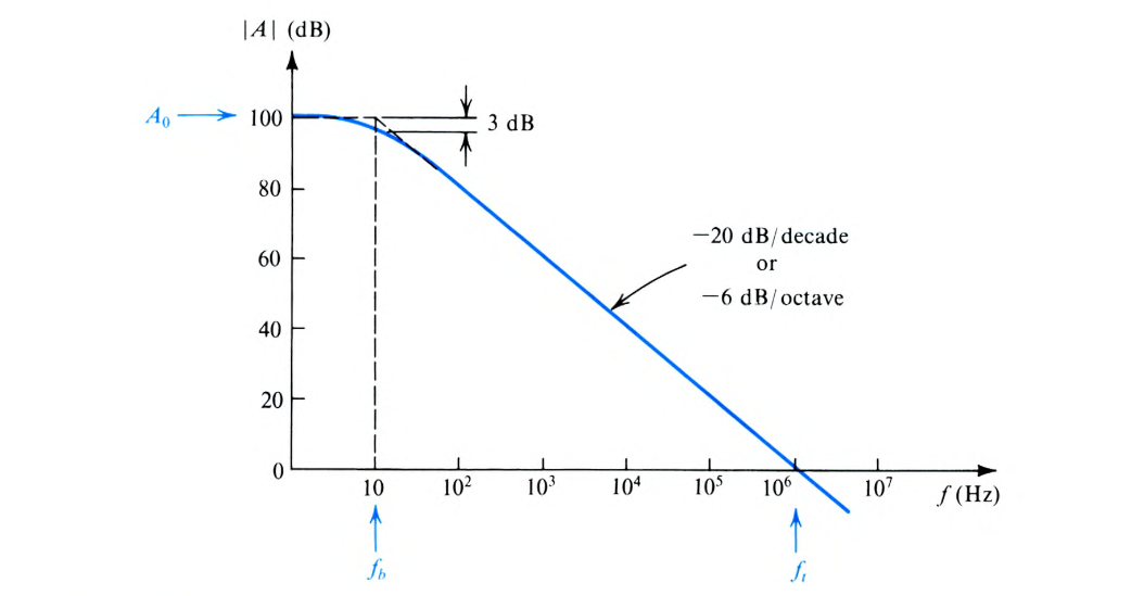
Some notes: while the gain is quite high at lower frequencies and at DC, it begins to decrease starting at a low frequency. The 20 dB per decade decrease is typical of internally compensated op amps, which have capacitors internally to cause an op amp gain with a STC low-pass response (this process is frequency compensation; i.e., it’ll have one pole). This is an intentional design choice, which results in stable op amps that don’t oscillate.

The gain function of an internally compensated op amp is given by:

$$A(j\omega )=\frac{A_0}{1+\frac{j\omega }{{\omega }_b}}$$

where $A_0$ is the DC gain and ${\omega }_b$ is the corner frequency (or the 3-dB point). For large frequencies:

$$A(j\omega )\simeq \frac{A_0{\omega }_b}{j\omega }=\frac{{\omega }_t}{j\omega }$$

We can denote the frequency at which the gain reaches unity (or 0 dB) by:

$${\omega }_t=A_0{\omega }_b$$

This is the unity-gain bandwidth and is an important parameter specified on data sheets. The gain bandwidth product is also an important parameter that shows up when we have inverting configurations.

The full-power bandwidth $f_M$ is a parameter used in conjunction with the slew rate. It tells us the maximum frequency at which a sinusoidal output begins to distort.

$$f_M=\frac{\text{SR}}{2\pi V_{o,\text{max}}}$$ $$\text{SR}={\omega }_M{V}_{o,\text{max}}$$

Circuit analysis

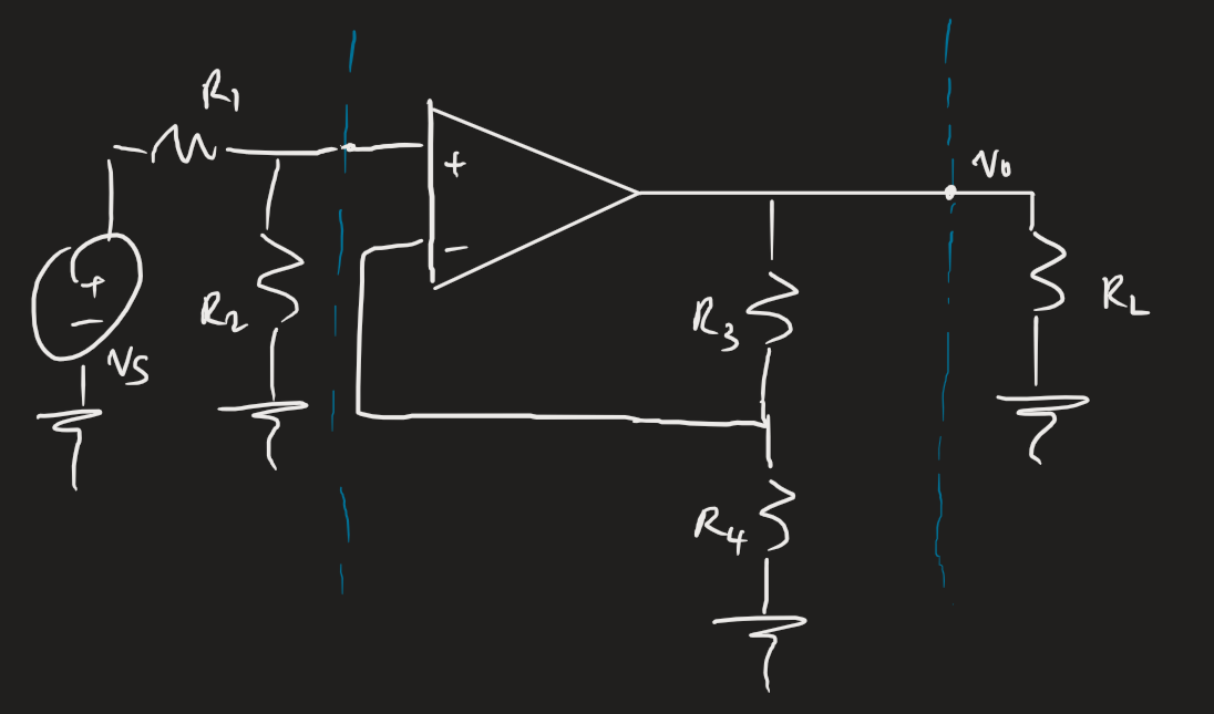
For an amplifier circuit like the one in the applications section, we have a voltage divider:

$$v_o=\frac{R_3+R_4}{R_3}{v}_n$$

i.e., the gain of the amplifier is determined solely by the resistors. For more intuition on how this happens, see this page.

Applications

There are a few common circuits we can build involving op amps. A non-inverting amplifier takes an input in the positive terminal: Conversely for an input plugged into the negative terminal, we have an inverting amplifier. We can also find this from the gain: if the gain is positive, it is non-inverting. From these two fundamental cases, we can build a variety of circuits with important applications:

• Buffer amplifier
• Analogue adder
• Comparator
• Transimpedance amplifier (current to voltage converter)
• Differentiator
• Integrator
• Low-pass filter
• Superdiode
• Astable multivibrator
• Schmitt trigger