Electric field

The electric field ($\vec{E}$) is a vector field, defined in terms of the electrostatic force exerted by a charge $q_1$ (or a distribution of charges) on another test charge $q_2$ at a given point. It’s measured in $\frac{N}{C}$ or $\frac{V}{m}$.

$${\vec{E}}_{12}=\frac{{\vec{F}}_{12}}{q_2}$$

We also commonly express the electric field in a different way, exerted by an isolated charge $q$ at an observation point $P$. Defined with respect to the origin, ${\vec{r}}^{\prime }$ points to the charge (source), and $\vec{r}$ points to the observation point. This is the most convenient formula — since we don’t need to convert to a unit vector.

$$\vec{E}(\vec{r},{\vec{r}}^{\prime })=\frac{1}{4\pi {ϵ}_0}\frac{q}{\Vert \vec{r}-{\vec{r}}^{\prime }{\Vert }^3}(\vec{r}-{\vec{r}}^{\prime })$$

Field lines are used to visualise the direction and magnitude of the electric field, where an increased density of field lines indicates a greater magnitude. The electric field vector is tangent to the electric field at any point.

From the formula, we can deduce that positively charged particle are sources of fields (i.e., they point away), and a negatively charged particle is a sink (i.e., they point in). Field vectors follow the principle of superposition, which allows us to discuss a system of charges.

Major definitions and equations

The electric flux is a flux integral, for the amount of electric field through a surface.

$${\Phi }_E={\iint }_S\vec{E}\cdot d\vec{S}$$

We relate the electric flux density with the field:

$$\vec{D}=ϵ\vec{E}$$

where $ϵ$ is the permittivity of the material. And relate the electric potential:

$$\vec{E}=\nabla V$$

where $\nabla$ is the gradient operator.

The electric field is curl-free:

$$\nabla \times \vec{E}=0$$ $${\oint }_C\vec{E}\cdot d\vec{l}=0$$

Due to charge distributions

For charge distributions, we have a very general set of steps:

1. Choose an applicable coordinate system.
   1. For example, for an infinite line charge or coaxial cable, we want to use the cylindrical system, since the field only depends on the distance from the line $r$ and not the relative height $z$ or angle $\phi$.
2. Pick one (arbitrary) differentially small point charge along the line. Find the expression for $dq$.
3. Find the resulting $d\vec{E}$ by the point charge $dq$ at the observation point (could be arbitrary).
   1. Wait! When you’re taking the norm of the vectors, neglect the angular terms. They don’t actually contribute anything.
   2. We can rationalise this by defining $\Vert \vec{r}\Vert =\sqrt{x^2+y^2+z^2}$. When you make the conversions to cylindrical and spherical, at no point do the angles show up.
4. Generalise the expression for $\vec{E}$ by integrating in the interval.
   1. If unit vectors that change with position are in the integral, we must convert to $\hat{x},\hat{y},\hat{z}$.
5. Compute the integral (analytically or numerically).
6. Check: does the result make physical sense?

We use a variation of Coulomb’s law for a differential charge element so it makes sense that we compute for a differential field:

$$d\vec{E}=\frac{1}{4\pi {ϵ}_0}\frac{dq}{\Vert \vec{r}-{\vec{r}}^{\prime }{\Vert }^3}(\vec{r}-{\vec{r}}^{\prime })$$

For example, let’s compute the field for an infinite line charge at an arbitrary point $\vec{r}=r\hat{r}+z\hat{z}$. We use cylindrical coordinates because the electric field only depends on $r$, not $\phi$ or $z$. The charge distribution is:

$${\rho }_l=\frac{dq}{dl}=\frac{dq}{dz}$$ $$dq={\rho }_{l}dz$$

We want to find $d\vec{E}$ at some point $⟨0,0,z^{\prime }⟩$.

$$\vec{r}=x\hat{x}+y\hat{y}+z\hat{z}$$ $$\vec{r}-{\vec{r}}^{\prime }=r\hat{r}-z^{\prime }\hat{z}$$

Substituting everything and integrating:

$$\vec{E}={\int }_{-\infty }^{\infty }\frac{{\rho }_{l}d{z}^{\prime }}{4\pi {ϵ}_0(y^2+(z^{\prime }{)}^2{)}^{\frac{3}{2}}}(r\hat{r}-z^{\prime }\hat{z})$$

Distributing the terms we get:

$$\vec{E}=\frac{{\rho }_l}{4\pi {ϵ}_0}(\hat{r}r{\int }_{-\infty }^{\infty }\frac{d{z}^{\prime }}{(y^2+z^{\prime 2}{)}^{\frac{3}{2}}}-\hat{z}{\int }_{-\infty }^{\infty }{z}^{\prime }\frac{d{z}^{\prime }}{(y^2+z^{\prime 2}{)}^{\frac{3}{2}}})$$

Some observations at this step:

• The Cartesian unit vectors never change, so they can be taken out of the integral.
• But the source coefficients ($z^{\prime }$, $d{z}^{\prime }$) will change as we integrate so we must leave them in.
• The $r$ term will simplify out to $2/y^2$. This is the result of some god awful trig substitutions.
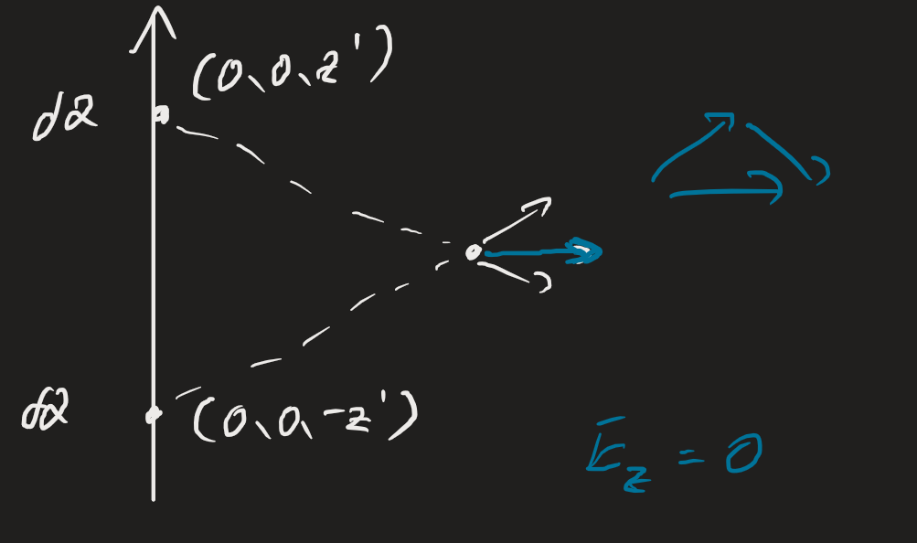
• More importantly the $z$ term is 0. This is because we’re integrating an odd function over a symmetric interval.
  • odd function/even function = odd function; more on that in the addendums section!

$$\vec{E}=\frac{{\rho }_l}{2\pi {ϵ}_{0}r}\hat{r}$$

Does this make physical sense? It’s dependent only on the radial distance from the line charge, so I’d suppose so.

Additional formulas

An alternate statement of the field exerted by an isolated particle, where $\vec{R}=\vec{r}-{\vec{r}}^{\prime }$ (points from source to observation point):

$$\vec{E}=\frac{kq}{\Vert \vec{R}{\Vert }^2}\hat{R}$$

Inside a conductor:

$$E=0$$

For an infinite sheet, where $\sigma$ is charge density in $C\cdot m^{-2}$:

$$E=\frac{\sigma }{2{ϵ}_0}$$

For between two equal and opposite plates with the same size of charge and opposite signs just outside the surface (where inside, $E=0$):

$$E=\frac{\sigma }{{ϵ}_0}$$

For a linear charge, where $\lambda$ is charge density in $C\cdot m^{-1}$ and where $r$ is the distance from the line:

$$E=\frac{\lambda }{2\pi {ϵ}_{0}r}$$

For a sphere with radius $R$:

$$E=\frac{kq}{R^3}r$$

We can relate electric field with current density and resistivity with:

$$\vec{E}=\rho \vec{J}$$

Addendums

The government sets legal limits for electric field emissions in controlled and uncontrolled environments with respect to an RMS voltage value.

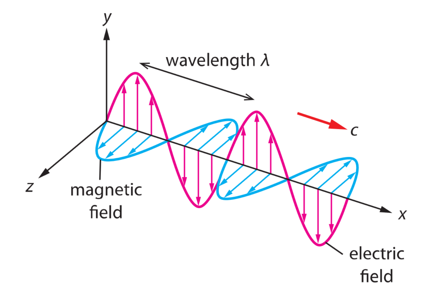
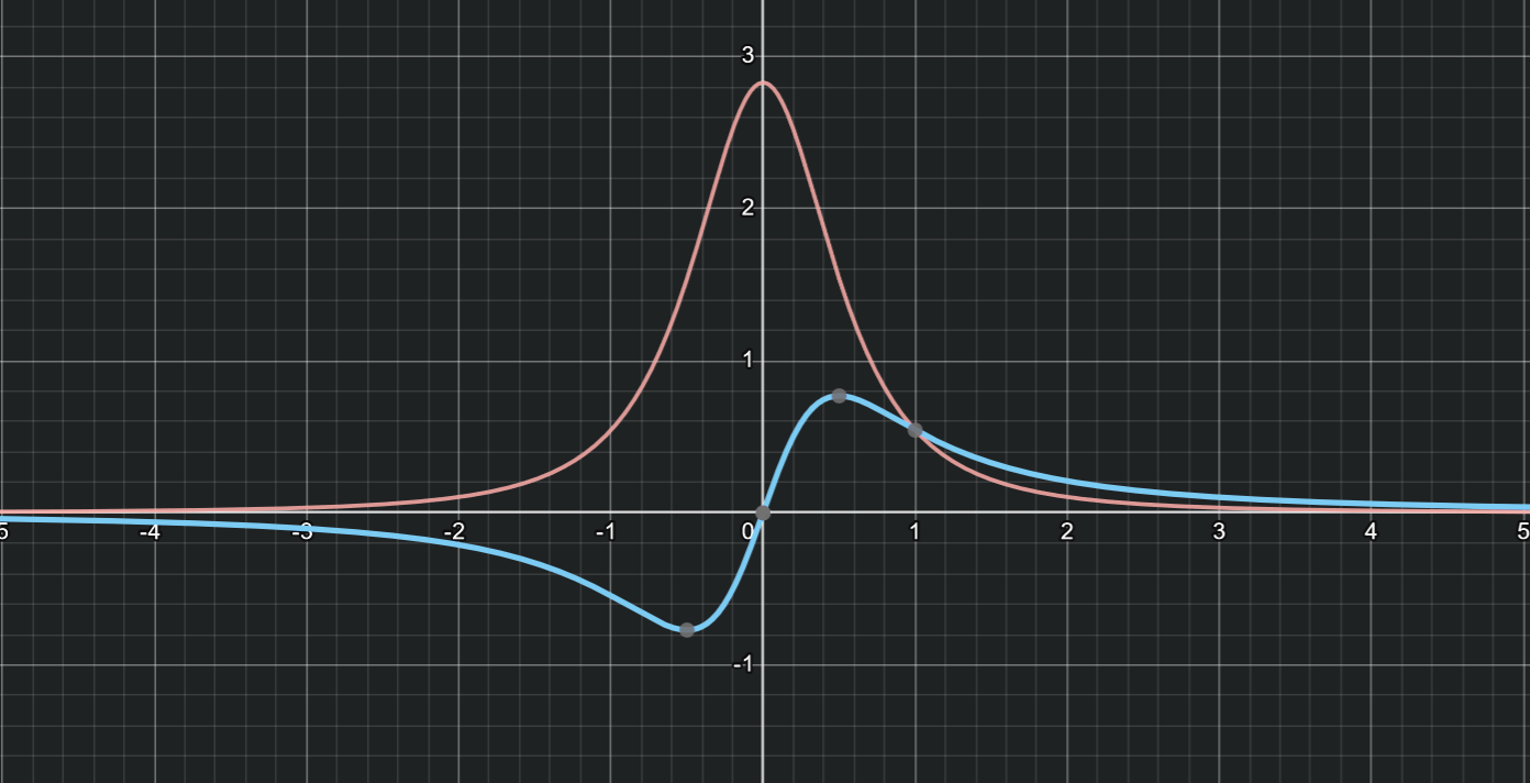
An oscillating electric field produces a perpendicular oscillating magnetic field, both at the speed of light in a vacuum. They’re collectively called electromagnetic waves, and are transverse waves. It’s a little difficult to convince yourself that a function that looks like:

$$\frac{1}{(y^2+z^{\prime 2}{)}^{\frac{3}{2}}}$$

is even over $\mathbb{R}$. The red curve is the above, and the blue curve is if we multiply by an additional $z^{\prime }$ term:

See also

• Magnetic field
• Gravitational field