Gauss' law

Gauss’ law states that the electric flux through an arbitrary closed Gaussian surface is equal to the charge enclosed by this surface. Mathematically, it is given by:

$$\oint {\oint }_S\vec{E}\cdot d\vec{S}=\frac{q_{\text{enc}}}{{ϵ}_0}$$

where ${ϵ}_0$ is the permittivity constant. Applying the divergence theorem:

$$\oint {\oint }_S\vec{E}\cdot d\vec{S}={\iiint }_v\nabla \cdot \vec{E}dv={\iiint }_v{\rho }_{v}dv=\frac{q_{\text{enc}}}{{ϵ}_0}$$

where $V$ is the volume enclosed by the Gaussian surface and ${\rho }_v$ is a volume charge density ($C\cdot m^{-3}$):

$${\rho }_v=\frac{dq}{dv}$$

Thus the differential form of Gauss’ law is:

$$\nabla \cdot \vec{E}=\frac{{\rho }_v}{{ϵ}_0}$$

Divergence theorem

A useful application of Gauss’ law is using the divergence theorem to find the electric field, since field calculations can get complicated. We only do this if $\vec{E}$ is irrotational (curl-free) and is caused by a symmetrical charge distribution.

Our Gaussian surfaces are cylinders, spheres, and rectangular boxes. The integrands are scalar values. Remember to use the delta function when looking at infinitely thin objects.

We follow a step-by-step process:

• Exploit symmetry. We either have spherical, cylindrical, or planar symmetry.
  • Determine what variables $\vec{E}$ depends on. In general for spherical and cylindrical, $\vec{E}=E(r)\hat{r}$.
  • Choose the right Gaussian surface for the problem.
• Compute the LHS and RHS of the divergence theorem.
  • Beware of cases where the Gaussian surface is within or outside the source. This happens when continuous charge distributions aren’t infinitely thin in one of the unit directions.
• Evaluate LHS = RHS to compute the field $\vec{E}$.

Tricky problems

There’s a broad class of problems where the charge distribution is defined continuously with some thickness. This means we need to evaluate multiple conditions (when the question asks to evaluate in all regions). For example, for a hollow ball with some thickness, we have three conditions:

• Within the hollow section
• Gaussian surface between the outer and inner layers
• Surface enclosing the entire ball

Superposition

Since vector fields follow the principle of superposition, we are able to break more complicated problems into smaller sub-problems and find a sum of contributions of sources.

Especially true is the idea of cavities. Maybe we have a void within a sphere — then we can subtract the field. This especially helps with different geometries — we can just find the sum.

Spherical symmetry

We use spheres for point charges and also spherical distributions. Thinking intuitively about a charge in free space, the field strength depends only on radial distance $r$ and not the angle; i.e., it depends on $r$ but not $\phi$ or $\theta$.

$$\vec{F}=F(r)\hat{r}=F(r)\hat{r}+F_{\theta }(r)\hat{\theta }+F_{\phi }(r)\hat{\phi }$$ $$0=F_{\theta }(r)=F_{\phi }(r)$$

The LHS of the divergence theorem will evaluate out to 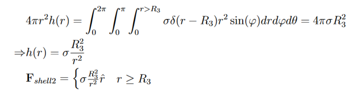$F(r)4\pi r^2$. Take note of what they’re doing above. This object isn’t actually centred at the origin, but because of the nature of spherical we essentially assume it’s centre is at $r=0$. Then the delta function is at $R_3$, the radius of the object.

To find the field at a given point, we use the Pythagorean theorem and some doable algebra. Our unit vector $\hat{r}$ can be decomposed:

$$\hat{r}=\frac{x}{r}\hat{x}+\frac{y}{r}\hat{y}+\frac{z}{r}\hat{z}$$

Cylindrical symmetry

Here, we determine the field generated by an infinite line charge along some axis with a line charge density $\lambda$.

$$\nabla \cdot \vec{F}=\rho =\frac{\lambda }{2\pi }\delta (r)$$

Using cylindrical symmetry (where the cylinder follows the line), the field only depends on $r=\sqrt{x^2+y^2}$.

$$\vec{F}=F(r)\hat{r}$$

A cylinder is most convenient for a Gaussian surface, where $z\in [0,h]$. When we do the computations:

• RHS should look like $\lambda h$. Intuitively, if $h$ metres are enclosed, and $\lambda =\frac{C}{m}$, then the charge enclosed makes sense. FOR A FILAMENT
  • As always, whenever we have the delta function, we should have a radius upper bound from $R+\Delta$ where $\Delta$ is arbitrarily small to sample the entire symmetry.
• LHS we compute the surface integral. However, the top and the bottom of the Gaussian cylinder should be perpendicular to $\hat{r}$, so we functionally only compute the surface integral for the curved surface. Remember the differential element includes an extra $r$.
  • It should always look like: $2\pi rhf(r)$

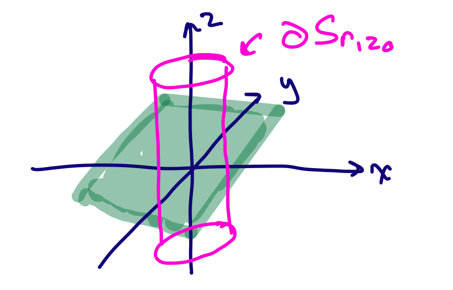
Planar symmetry

For planar symmetry, we can use either cylinders or prisms. Cylinders in general look like the easiest to use. In this case, we instead have the cylinder tops and bottoms parallel to the plane:

$$S=\{x^2+y^2=r^2;z\in [-h,h]\}$$

The field only depends on the distance away from the plane, i.e., for the cylinder it only depends on $z$ and not $r$ or $\theta$.

$$\vec{F}=F(z)\hat{z}$$

As a result, the cylinder body is now perpendicular to the field, and the tops and bottoms are actually evaluated this time.

Further applications

We can use Gauss’ law to derive Coulomb’s law for a point charge and find the electric field. This is an example of the spherical symmetry above. We enclose the particle in a Gaussian sphere that is centred on the particle. Then, the electric field has the same magnitude $E$ at any point on the sphere, simplifying the integration.

$${ϵ}_0\oint \vec{E}\cdot \overrightarrow{dA}=q_{enc}$$ $${ϵ}_0\oint EdA=q_{enc}$$

The area is given by $A=4\pi r^2$, so we simplify:

$${ϵ}_{0}E(4\pi r^2)=q$$ $$E=\frac{q}{{ϵ}_{0}4\pi r^2}$$

which is exactly Coulomb’s law.