Recurrent neural network

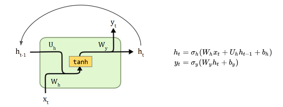
In deep learning, a recurrent neural network (RNN) is a neural network architecture that takes in a variable-sized sequential input and can remember things over time (i.e., it has a memory/state). This is stored in a context vector with an initial blank slate. It is an example of an autoregressive model, which is sequential. 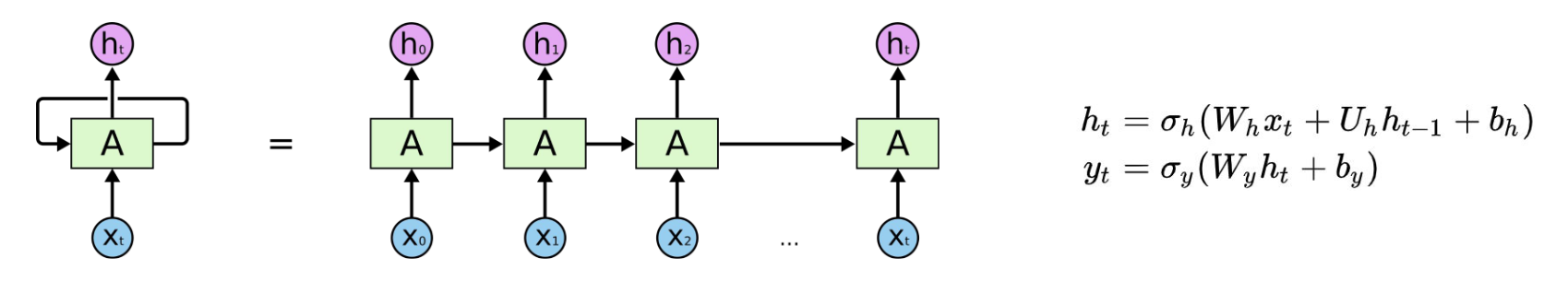The hidden state (in the context vector) is updated based on previous hidden states and the input (for NLP, often a GloVe embedding), i.e., hidden = update(hidden, input). This is done with the same neural network as before (weight sharing), and we effectively iterate through the input tokens until we’re at the end. Then, the last hidden state is input into a prediction network (an MLP).

Many real-world problems deal with sequential inputs/outputs of varying sizes. Text, video, time-series data, financial data.

General problem: we can’t make use of vectorisation or CUDA because RNNs are sequential in nature. This motivates the idea of transformers.

Premise

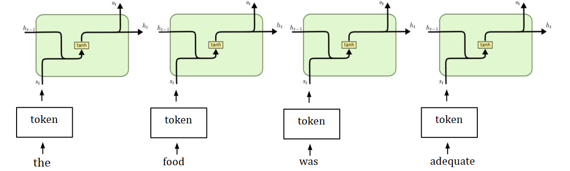
In a sequence, we don’t want to learn different weights for every token. RNNs use a shared neural network to update its hidden state, which reuses the RNN module for every token in the sequence. It keeps the context of the previous tokens encoded in the hidden state.

The forward pass in an RNN is basically a fully-connected NN. Each module is a particular sequence of NN modules, and we can unroll it to visualise how the RNN processes sequential data. Deep RNNs (with a long sequence) aren’t good at modelling long-term dependencies. They’re also hard to train due to exploding/vanishing gradients. If we represent an individual and every time-step as:

$$h_t=W_h{h}_{t-1}$$ $$h_t=(W_h{)}^t{h}_0$$

Then we have exploding gradients if $|W_h|>1$ and vanishing gradients if $|W_h|<1$. Solution? We clip the gradient by setting a threshold to it if it begins to vanish/explode. We can also preserve the hidden state/context over the long-term, i.e., a skip connection every so often, and not to every previous state.

Gating mechanism

We can approximate skip connections to previous states by learning to weigh previous states differently instead (soft skip connections). These are done via gates that learn to update the context selectively.

The gating mechanism controls how much information flows through. If $\vec{X}$ is a vector, then, we can apply an activation function $\sigma$ or a neural network:

$$f(x)=\vec{X}\cdot \sigma (\vec{X})$$ $$f(x)=\vec{X}\cdot \text{NN}(\vec{X})$$

Architectural variations

Variations on vanilla RNNs include LSTMs and GRUs, which make use of gates. In general, LSTMs and GRUs can be trained on longer sequences and are much better at learning long-term relationships. They’re also easier to train (need more epochs) and achieve better performance than vanilla RNNs.

We can stack RNN layers to learn more abstract representations. The first layers’ representations are better for syntactic tasks, and the last layers perform better on semantic tasks.

Some RNNs are also bidirectional, i.e., where they rely on the past, present, and future (unlike in typical RNNs). This is necessary for tasks like machine translation.

Other tasks require different subtle architectural changes. 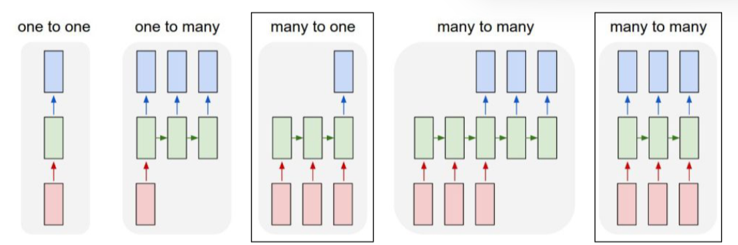Sequence-to-sequence RNNs learn to generate new sequences. We can denote the end of a sequence with an eos token. To generate a given sequence in the training set (i.e., bos right eos), we can feed the RNN with a bos beginning of sequence token and compare each character’s prediction. This loss is computed with cross entropy.

A variation on this is called teacher forcing. The idea: to make training more efficient, we can force the RNN to stay close to the ground-truth. Even if it predicts a bad token, we pass the ground truth as the next input.

At inference-time, we make use of certain strategies for text generation. We can’t blindly select the token with the highest probability, because we don’t necessarily want deterministic behaviour. A greedy approach just results in a lot of grammatical errors. We can use three sampling strategies to sample from the predicted distributions.

• Greedy search takes the token with the highest probability as the generated token.
• Beam search looks for a sequence of tokens with the highest probability within a window.
• Softmax temperature scaling helps solve over-confidence in neural networks by scaling the input logits to the softmax with a temperature.
  • A low temperature has larger logits with more confidence. It generates higher quality samples with less variety.
  • A high temperature has smaller logits with less confidence. It has the opposite.
  • Conceptually, the temperature is similar to the idea of simulated annealing. A high temperature indicates large levels of exploration compared to a low temperature.

In code

In PyTorch, a vanilla RNN layer is specified by:

self.rnn_layer = nn.RNN(input_size = 50,
				  hidden_size = 64,
				  batch_first = True)

But we typically express an actual RNN model with the above as an intermediate layer. The layer prior may be an embedding (i.e., a vector embedding), and the layer after may be another RNN layer or a fully connected layer.¹

Footnotes

1. See lab 5 from APS360. ↩