Search is a fundamental technique in computer science, including in AI. It’s useful because it’s a general problem-solving technique, can outperform humans in some areas (games like chess or go), and some aspects of intelligence can be formulated as a search problem. However, we can only solve a problem as a search problem once we’ve correctly formulated it.
Formulation
The components of a search problem:
- State space — a state is a representation of a configuration of the problem domain. The state space is the set of all states included in our model of the problem.
- Initial state — the starting configuration.
- Actions (or successor function) — allowed changes to move from one state to another.
- Goal states (or goal test) — configurations one wants to achieve.
- Optional cost associated with each action.
- Optional heuristic function to guide the search, which represents how close we are to a goal.
- A solution to the problem is a sequence of actions/moves that can transform the initial state to a goal state (optionally minimising the total cost).
In search problems, we use problem-specific state representations and heuristics. We’re generally concerned about determining paths from the current state to goal states. And we view states as black boxes with no internal structures. We also generally use a generic algorithm.
Note: search problems can get more complicated — for example, the state transition may not be deterministic, we may not have full knowledge of every state (for example, prize is behind door 1, 2, 3). In these cases, we need to assign probabilities to each outcome and solve this way.
We can represent the state space visually with state space graphs (much like FSM state diagrams), where vertices are states, and directed edges are transitions resulting from the successor functions. The goal test is a set of goal states. Each state in a state space graph is unique. We rarely construct the full graph in memory (often too big).
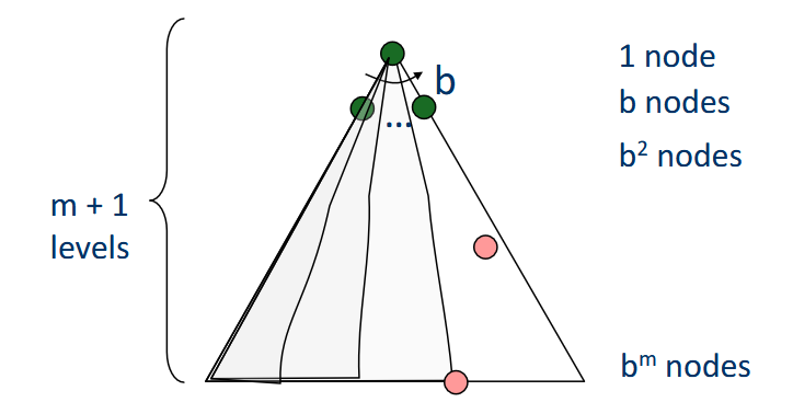
A search tree reflects the behaviour of an algorithm as it walks through a search problem. The initial state is the root node, and children correspond to successors. A node in a tree corresponds to a path that achieves the state — result is that the same state may appear many times in a search tree. Like with state space graphs, we never build the entire tree. Note also that for cyclic state graphs, we have a resulting infinitely large search tree.
There are a few important definitions:
- Branching factor , which is the maximum number of successors of any state.
- Max depth , which is the length of the longest path.
- Depth of the shallowest goal node , which is the length of the shortest solution.
unsorted notes
- UCS: uniform cost search — useful when actions correspond to a cost
- infinite branching factor: generally prefer DFS to BFS. but neither are really appropriate b/c solution state may be in right-side of tree and we’ll likely run out of memory
- iterative deepening search: DFS space with BFS time/finding length optimal solution
- completeness? yes if branching factor is finite
- optimality? length optimal
- space
- time
Algorithms
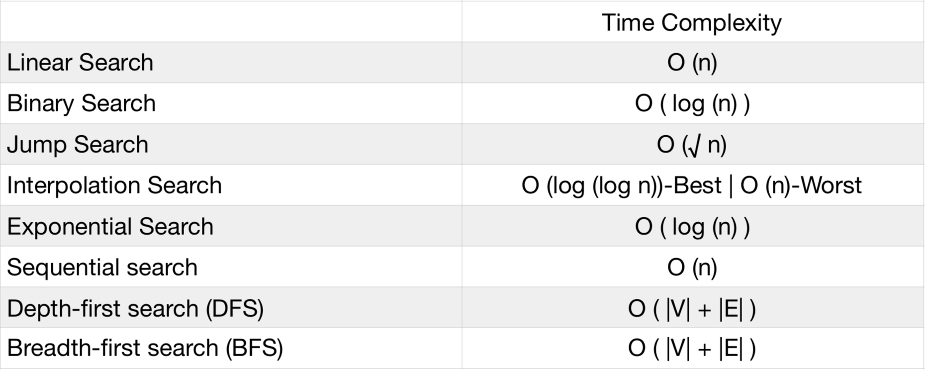
Searching algorithms find a value inside a given data structure. Common searching algorithms are applied on arrays, linked lists and binary trees, but more generally graphs.
 When searching through graphs, we often use a data structure to store the frontier, i.e., the nodes that we have not checked yet. Then, when we consume a frontier node, we insert its children back into the frontier. Three choices of data structure make sense:
- A priority queue, which pops the node with the minimum cost, used in Dijkstra’s algorithm.
- A FIFO queue, used in breadth-first search.
- A stack (or LIFO queue), used in depth-first search.
Sub-pages
- Binary search
- Uninformed search
- Depth-first search
- Breadth-first search
- Iterative deepening search
- Dijkstra’s algorithm (uniform-cost search)
- Heuristic search