Small signal modelling

Small signal modelling is an analysis technique used to approximate non-linear behaviour with a linear equation. This is especially useful in analysing non-linear circuit elements, like diodes or transistors. More on that at a dedicated page.

Premise

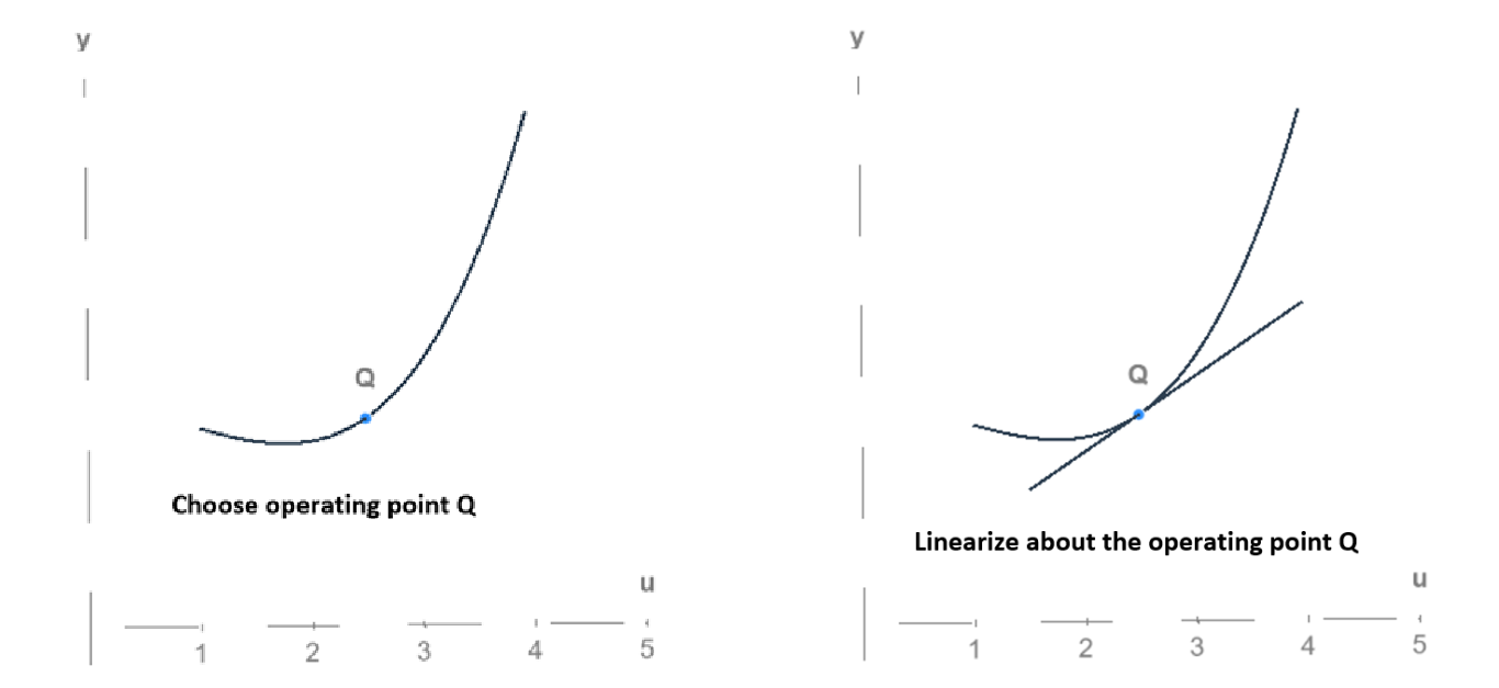
The general procedure for small signal modelling is to take some function $y=g(u)$ with some operating point $Q(u,g(u))$ (also called the bias point or quiescent point) along the curve. We then take a linear approximation about the point, and apply some small change in a time varying input to find a small signal output. The $u$-component of the point is $U$ and the $y$-component of the point is $Y=g(U)$. Consider these constant values.

Visually: 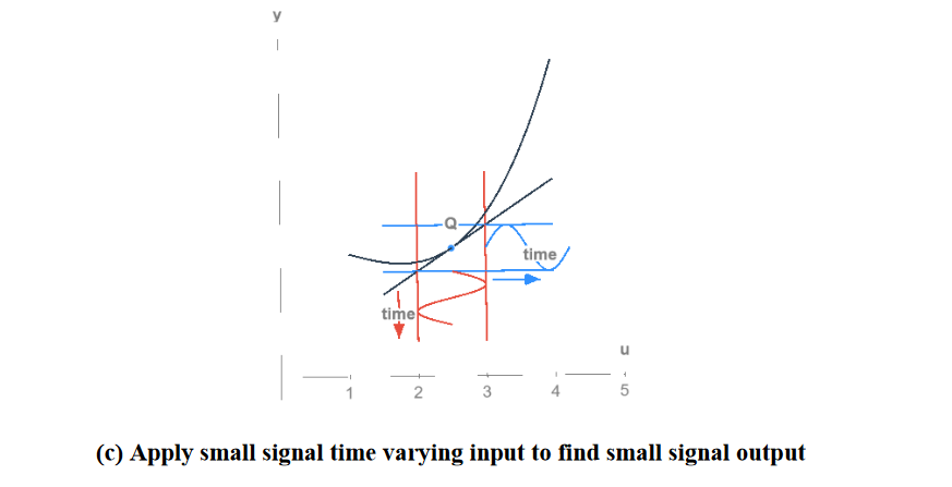What does this mean though? Because we use a linear approximation, we’re interested in small variations about the operating point $Q$. Because we vary by a small amount of time about $U$, we define some new value of the input variable $u$ with respect to a small change in $u$ ($\Delta u=\hat{u}(t)$):

$$u=U+\Delta u+U=\hat{u}(t)$$

The result of this is that our output signal $y$ will also vary by a small amount about $Y$. In the relation below, $U$ is some constant (probably related to the operating point) and $t$ is time.

$$Y+\hat{y}(t)=g(U+\hat{u}(t))$$

Our goal: to find the relationship between $\hat{y}(t)$ and $\hat{u}(t)$ for some function $g(u)$, i.e., how does $y$ vary as a function of time for some small change in the input $u$?

Note from the above graph that we overlay another time-varying curve (i.e., we add a new curve wrt time that wasn’t there before).

Definitions

There’s a lot of notation and terminology thrown around:

• Operating point ($Q$) — The point we linearise about; in circuits, this is a DC offset value. $Q$ has two parameters in $u,y$ space: $(U,g(u))$.
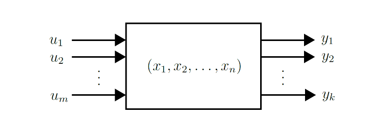
• State variable ($x$): variable in a first-order derivative $\frac{dx}{dt}$. As a result of the input variables varying, the state variables vary slightly about a state variable equilibrium point $X_1\dots X_n$.
• Input variable ($u$): variable representing an excitation signal, like an input voltage or current source. They are small input signal variations $u_1\dots u_m$ that vary about an equilibrium point $U_1\dots U_m$.
• Output variable ($y$): function of the state variable and input variable, $y=g(x,u)$. As a result of input variables varying, the output variables vary about an equilibrium point $Y_1\dots Y_k$.
• State-space model: links state variables, excitation inputs, and output variables together, with $n$ first-order non-linear differential equations.

Procedure

We have a multi-step procedure:

• Step 1: Convert space variable equations into state space equations (take the derivative). Expand the state space equations and output equations in terms of $n$, $m$, and $k$ using the first-order Taylor series. The result are linear differential equations and linear output equations. Oftentimes we are given these equations and can safely skip this step.
• Step 2: Determine equilibrium solutions:
  • Determine the equilibrium for the state space equations $X_1,X_2$. Set the derivatives to 0 and solve for whatever $x_1$ and $x_2$ are.
  • Determine the equilibrium for the output variables $Y_1,Y_2$. Into the output equation, input the equilibrium values we found for $X_1,X_2$ above and the equilibrium input variables that we were given to find $Y_1,Y_2$
• Step 3: For the perturbations in the state space equations, we can take the equations, and evaluate the respective Jacobians at the equilibrium points.

$$\left[\begin{array}{c}\frac{d{\hat{x}}_1}{dt}\\ \frac{d{\hat{x}}_2}{dt}\end{array}\right]={\text{J}}_f\left[\begin{array}{c}{\hat{x}}_1\\ {\hat{x}}_2\end{array}\right]+{\text{B}}_f\left[\begin{array}{c}{\hat{u}}_1\\ {\hat{u}}_2\end{array}\right]$$ $$\left[\begin{array}{c}{\hat{y}}_1\\ {\hat{y}}_2\end{array}\right]={\text{J}}_g\left[\begin{array}{c}{\hat{x}}_1\\ {\hat{x}}_2\end{array}\right]+{\text{B}}_g\left[\begin{array}{c}{\hat{u}}_1\\ {\hat{u}}_2\end{array}\right]$$

Side notes

For the single variable case, our general procedure takes 4 steps:

• Step 1: write $y$ as a function of the operating point $Y$ and some small variance.

$$Y+\hat{y}(t)=g(U+\hat{u}(t))$$

• Step 2: Expand the right hand side of the expression up to the first-order Taylor series. Evaluate the expression at the operating point $Q(U,Y)$.

$$g(U+\hat{u}(t))\approx g(U)+\frac{dg}{du}{|}_{u=U}\hat{u}(t)$$

• Step 3: Equate the left-hand side with the expansion we just did.

$$Y+\hat{y}(t)=g(U)+\frac{dg}{du}{|}_{u=U}\hat{u}(t)$$

• Step 4: Determine the small signal model by expressing in terms of $\hat{y}(t)$ on one side. In this case, $Y=g(U)$.