Level curves and surfaces

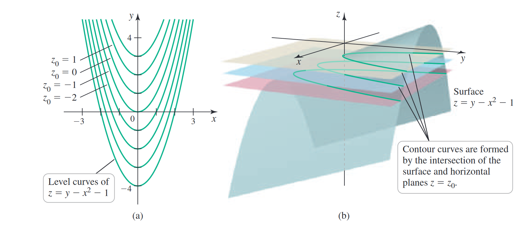
The easiest analogy for level curves is as a topographic map for the function. We want to map $z=f(x,y)$ for constant values of $z$ onto the $xy$ plane, i.e., by projecting the intersection between $z$ and a plane at $z=c$.

So for different values of $z$, we take a plane and graph down contour curves (i.e., the intersection curve) between the multivariable function and the plane. The values of $z$ are equidistant — if they are bunched up, the function is changing rapidly.

Level surfaces

Level surfaces project a function in ${\mathbb{R}}^4$, $w=f(x,y,z)$ onto the $xyz$ axes. We similarly take different constant values of $w$, then plot the three-dimensional projections.

See also

• Trace
• Graphing of functions