Convolutional neural network

In deep learning, convolutional neural networks (CNNs) are a popular type of neural network that use the convolution. CNNs work best with data that has a grid-like topology, like for vision applications. This is because of the convolution’s properties and use in image processing.

Architecture

CNNs consist of two big systems in sequence. The first is the encoder, which applies the convolution and some other functions (including a pooling layer after every convolution). The encoder’s output is flattened into a classifier (which can be a typical MLP). The classifier’s output is fed into softmax, which effectively allows it to classify between $n$ different classes.

The part where these two systems intersect is an embedding, a learned set of visual features that represent the image, i.e., CNNs learn something general about representing images through training.

What makes CNNs different from MLPs is that:

• They’re not fully connected, but instead locally connected. We have different filters for small regions of the image, since the spatial correlation of features is local.
• We also share weights, to detect the same local features across the entire image. This means that overall we have less weights than a fully connected MLP.
• The weights learned are the kernel values.

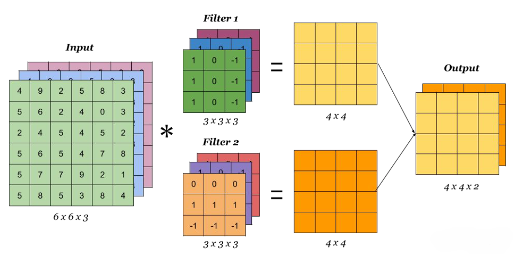
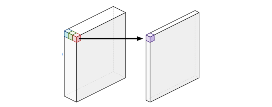
As the CNN continues layer by layer, the filter depth must increase (i.e., each convolution operation produces a deeper sub-image to operate on). The feature map height and width also decreases (i.e., the convolution operates on a smaller sub-image). Since we usually have RGB(A) channels, our kernel is functionally a 3-dimensional tensor, i.e., our kernel has one dimension for each colour channel. Note that the output for a multidimensional kernel is always a single value, even if we operate on multiple channels. The different output channels is determined by multiple different kernels.

Note also that each distinct kernel has a distinct bias term.

Computations

ML algorithms implement a variation of the convolution called the cross-correlation.

$$S[i,j]=(K\ast I)[i,j]=\sum _{n=-\infty }^{\infty }\sum _{m=-\infty }^{\infty }K[m,n]I[i+m,j+n]$$

For a better understanding of how the DT 2D convolution works, see this page.

We still have a forward and backward pass. We initialise the kernel values randomly. In the forward pass, we convolve the image with the kernel. In the backwards pass, we update the kernel using gradients. The number of parameters is given by the product of: input channels, output channels, and (kernel size)²

We sometimes add zeroes around the border of the image before convolving, called zero padding. This is to keep the height and width consistent with the previous layer and to keep information around the border of the image. The stride is the distance between two consecutive positions of the kernel, which allows us to control the output resolution. The output resolution is given by:

$$o=\lfloor \frac{i+2p-k}{s}\rfloor +1$$

where $i$ is the image dimension, $k$ is the kernel size, $p$ is the padding size, and $s$ is the stride size. This needs to be computed twice (one for each dimension) if the kernel or image aren’t square.

We use pooling to consolidate information at the end of our CNN. Pooling applies a simplification, according to a small-sized kernel.

Addendums

We can also do a pointwise convolution as a pixel linear transformation. We can learn to map CNN features into a higher or lower dimensional space, good for learning compact representations/compression. They’re used in all modern CNN architectures. Convolutions are great because unlike MLPs, the inputs can have varying spatial dimensions. MLPs require all inputs to have the same dimensions.

Kernels

Inception blocks use a mixture of multiple kernel sizes on one layer. Note that kernels don’t actually need to be larger than 3x3,¹ because multi-layered convolutions can approximate the results of any arbitrarily larger sized kernel.

What does a 1x1 convolution (kernel size 1) even do? It’s a pixel-wise non-linear transformation used to change the dimensionality of the filter space. Oftentimes it’s used to reduce the number of depth channels, which helps code run faster; it’s not used to extract features.

The neural network can “choose” which colour channels to look at with a 1x1 convolution, instead of brute force multiplying everything.

In code

In PyTorch, we use the torch.nn.Conv2d() function to specify a convolutional layer. It has the following parameters:

• in_channels specifies the number of input channels to a convolution. From an RGB image, we use 3 channels. The number of channels must be an int.
• out_channels specifies the number of output channels to a pooling layer.
• kernel_size specifies how large the kernel is (from a square). This parameter and the below can be an integer or a tuple.
• stride and padding are analogous to their theoretical counterparts. By default, stride=1 and padding=0.

We can also implement pooling functions. torch.nn.MaxPool2d() specifies a 2D pooling function, with parameters kernel_size and stride. As always, we want a pooling layer after a convolution layer. Our convolution layers should match the number of input/output channels as necessary.

See also

• LeNet
• AlexNet
• GoogLeNet
• Graph convolutional network

Footnotes

1. Result from the VGG network in 2014. ↩