Convolution image processing

The multidimensional discrete-time convolution finds significant use in image processing and computer vision. We define:

$$S[i,j]=(I\ast K)[i,j]=\sum _{n=-\infty }^{\infty }\sum _{m=-\infty }^{\infty }I[m,n]K[i-m,j-n]$$

The first argument $I$ is called the input, and the second argument $K$ the kernel. The output $S$ is the feature map. Images function as the input, and parameters adapted by our algorithm function as the kernel.

In most image applications (including ML), both the input and kernel are multidimensional arrays/parameters because we often have RGBA channels. In practice, the summation is also bounded because the image dimensions are also bounded.

Computations

By hand

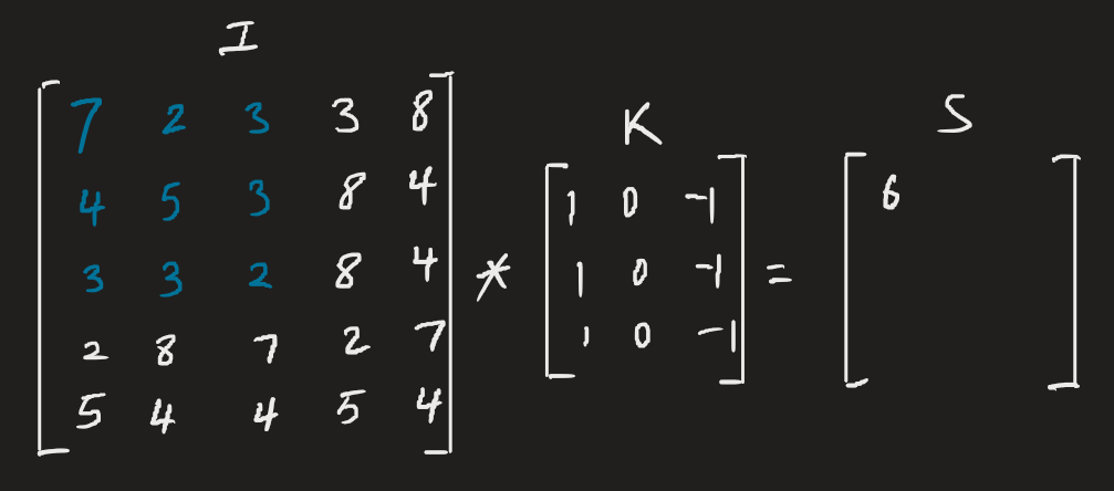
Practically speaking: for a 2D image, we apply the kernel to a subset of the image, then multiply elementwise for each element of the kernel/sub-image. This is output to a new 2D image, then the kernel is moved.

Elementwise multiplication is done here. Note that $S$ is a $3\times 3$ matrix, so the kernel slides to the right twice, and down twice. This doesn’t implement kernel flipping.

Numerically

Note that because the convolution is commutative, the following is valid:

$$S[i,j]=(K\ast I)[i,j]=\sum _{n=-\infty }^{\infty }\sum _{m=-\infty }^{\infty }K[m,n]I[i-m,j-n]$$

This is usually more straightforward to implement in a software library, because $m,n$ vary less. Note that commutativity means we flip the kernel relative to the input image.

i.e., as $m$ increases across the image, we move rightward through the image but leftward through the kernel.

This is not a very important result. Deep learning libraries instead implement the cross-correlation function, which functions the same as the convolution without flipping the kernel. For convenience, this is also called the convolution.

$$S[i,j]=(K\ast I)[i,j]=\sum _{n=-\infty }^{\infty }\sum _{m=-\infty }^{\infty }K[m,n]I[i+m,j+n]$$

The job of ML algorithms is to learn the appropriate kernel values.

Variants

Some variants of the convolution are:

• Transposed convolution
• Inverse convolution

Results

In traditional image processing, kernel filters can be used to perform practical steps. For instance, a kernel with uniform values less than 1 will blur out intensities in an image:

$$K=\frac{1}{9}\left[\begin{array}{ccc}1& 1& 1\\ 1& 1& 1\\ 1& 1& 1\end{array}\right]$$

Carefully engineering other filters, we can also:

• Detect vertical edges
• Detect horizontal edges
• Detect blobs (i.e., regions that differ in properties like brightness or colour compared to surrounding regions)
• Face detection

But since these filters are hand-crafted (like other DSP algorithms), we now use convolutional neural networks for computer vision applications, which can automatically craft features. Classical computer vision used multi-stage, careful engineering of kernels to achieve practical effects.

Maps

As mentioned above, the output of the multidimensional DT convolution (or a convolutional layer in a CNN) is called the feature map. It describes the learned representations (features) in the images.

The receptive field describes all the elements from all previous layers that may affect the calculation of an element during forward propagation. This may be larger than the actual input size, and largely describe edges and shapes.