Second-order ordinary differential equations are ODEs where the highest derivative in the equation is the second derivative. These can get pretty difficult to solve, but are very common in engineering, like in oscillatory systems and Kirchhoff’s laws.
If the other side of the equation is zero, it is homogeneous. Otherwise it is non-homogeneous. Recall that to solve a non-homogeneous ODE, we must solve for the particular solution. Methods are detailed in that page. For linear homogeneous second-order ODEs, we can use reduction of order.
By theorem, the general solution (or solution space) of a second-order linear homogeneous ODE with constant coefficients is two-dimensional.
Solutions
For second-order linear ODEs with constant coefficients, our characteristic equation is always a polynomial of degree 2 (i.e. a quadratic), so we have three possible cases: two real roots, one repeated real root, and two complex roots. Our candidate solution will involve .
For two real roots, we have the general solution:
For one repeated real root, since one term will be linearly dependent of the other, we multiply one term by . This follows as an extension of reduction of order, but the details aren’t important.
Complex roots
For two complex roots, where , , as a result of Euler’s formula:
Note that and must be unitless: so and represent frequencies. We call the neper frequency and the radian frequency.
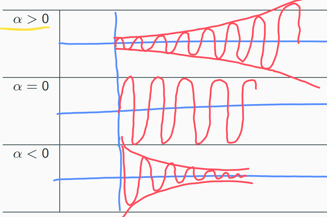
Looking closer, for , we have the sinusoidal terms bounded by an exponential, so they will scale accordingly. For , we have an unbounded sinusoid. For , they are bounded by an exponential decay function.
Parameters
We introduce two new parameters related to the time response:
where describes the undamped natural frequency. describes the damping ratio.
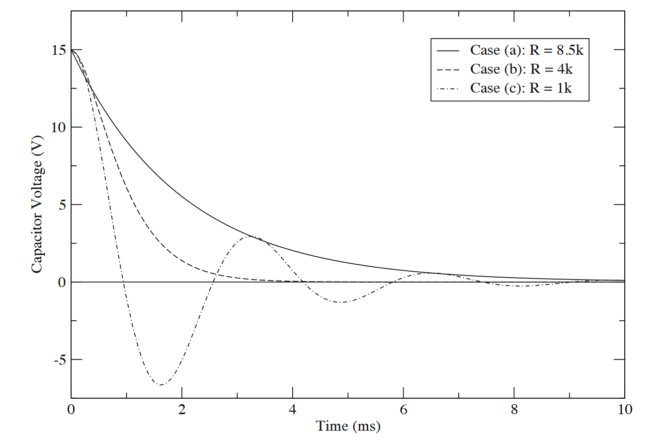
Graphically speaking, for a homogeneous ODE, we should get the following graph. Case (a) describes an overdamped system.